Category: Blog

Blog

Loss function in Machine Learning

Loss function in AI and Deep learning

Loss function in AI and Deep Learning measures how correctly your AI model predicts the expected outcome. A classroom image to explain loss function in AI

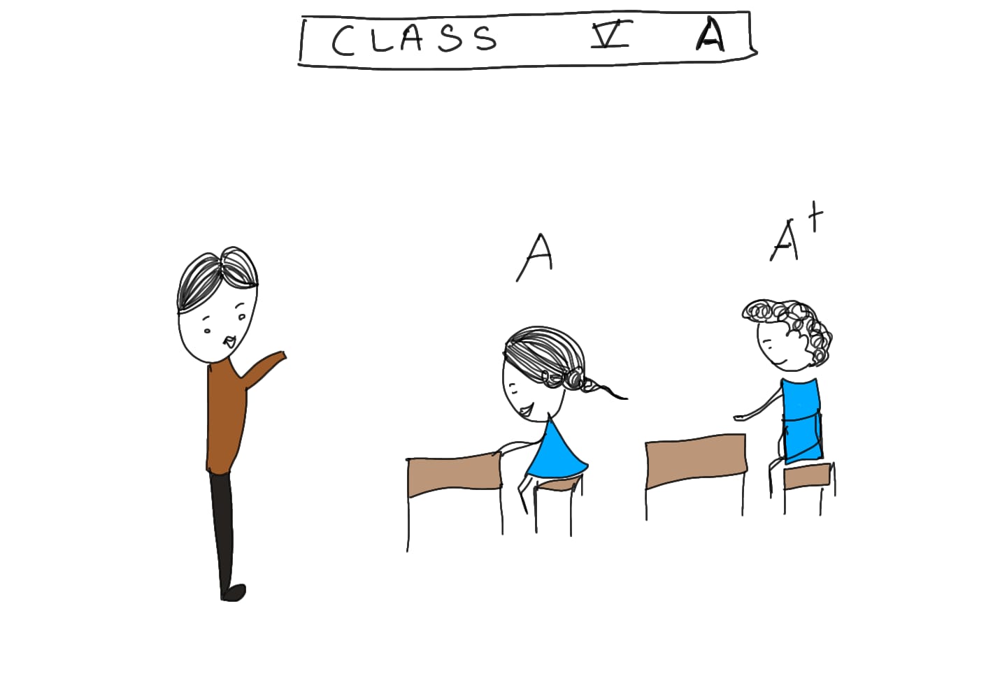
We use different loss functions for regression analysis and classification analysis.

Let us understand through a simple example.

Consider you have created an AI model to predict whether the student fits in Grade A, A+, or A-. It calculates a few parameters like marks of all the subjects in theory, practical, and projects to predict the grades.

The system may not predict correct grades in the first go resulting in a loss. This loss is used in backpropagation to reduce faulty predictions.

Learn how to get better accuracy by using Activation functions – Click here 

Loss = Desired output – actual output (Expected – reality)

If your loss function value is low, your model will provide good results. Thus, we should try to get a minimum loss value (high accuracy).

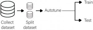
After forward propagation, we find the loss and reduce it. Now, let us learn about different types of loss functions.

How to reduce loss? What is loss function in machine learning? What is cost function?


We calculate the loss using the loss function and cost function.

The terms cost and loss functions almost all refer to the same meaning. The cost function measures error on a group of objects, and the loss function deals with a single data instance.


Loss function: Refers to error for a single training example.
Cost function: Refers to an average loss over an entire training dataset.

Do you recollect the above example to grade the students? The loss function evaluates the model’s performance for one student; the cost function evaluates the performance of the entire class. Therefore, to optimize our model, we need to minimize the value of the cost function.

We use different types of loss functions for different types of Deep learning problems.

There are two types of problems in supervised Deep Learning
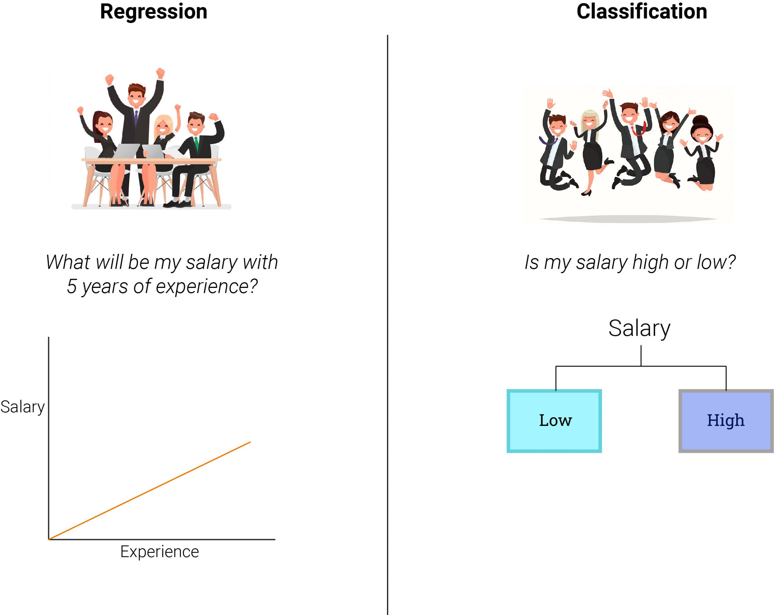
Regression and classification

Regression

The salary of an employee depends on the experience the employee has. Consequently, salary is a dependent variable known as the target, and experience is an independent variable known as the predictor.

Regression analysis explains to us how the value of the dependent variable changes based on the independent variable. It is a supervised learning technique that helps us to find the correlation between variables and predict the continuous output variable. We use it for prediction, forecasting, and determining the causal-effect relationship between variables.

The loss functions used for regression examples –

We use distance-based error as follows:

Error = y – y’
Where y = actual output & y’ = predicted output

The most used regression cost functions are below.


1. Mean error (ME):

Mean error = Sum of all errors /number of training examples

= {( Y1 – Y1’) + ( Y2 – Y2’ ) + ( Y3 – Y3’ ) + ….. + ( Yn – Yn’)}
n
= (+100 + -100) / 2
= 0 / 2 = 0.

· Here, we calculate the error for each training data and derive their mean value.
· The errors can be positive and negative,  sometimes resulting in a zero mean error for the model.
· Therefore, this is used as a base for other cost functions.

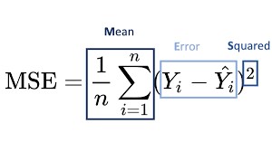
2. Mean Squared Error (MSE)


We use the mean squared error to get rid of the zero mean error. MSE is also known as L2 loss. We consider the square of the difference between the predicted and the actual value.

Mean Squared Error MSE in Regression Analysis

Advantages

· We can penalize the tiny deviations in predictions compared to MAE.
· It has only one local minima, and one global minima; converges faster, and is differentiable.

Disadvantages

· It is not robust to outliers. These outliers contribute to higher prediction errors, and squaring them further magnifies the error.
This equation is quadratic, resulting in gradient descent.

Info byte


OUTLIERS:


Say if we are predicting the value of the salary of a candidate. The salary depends on the experience of the candidate. And for that, we have a dataset of the salary and experience. Here, the salary might be very high or low in some cases, irrespective of their experience. These exceptions are known as outliers in a dataset that contribute to higher prediction errors.

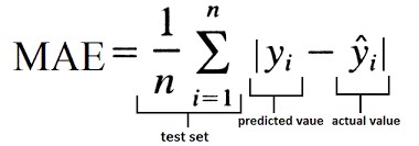
3. Mean Absolute Error (MAE)


MAE eliminates the ME shortcoming differently. Here, we consider the absolute difference between the actual and predicted value. It is measured as an average sum of absolute differences between actual and predicted values. MAE is also known as L1 loss.
MAE is Mean absolute error in regression analysis

Advantages

· Robust to outliers since we take the absolute value instead of squaring the errors.
· Gives better results even when the dataset has noise or outliers.

Disadvantages

1. It is a time-consuming function.

4. Huber Loss


Say we have salary values of 100 employees. Out of which, 12 employees have very high salaries, and 12 have very low salaries. Though these extremes fit in the definition of outliers, we cannot ignore them as they are about 25 percent of the dataset.
What do we do here? We use the Huber loss function.

The Huber loss function can be used to balance between MSE and MAE. It is a blend of mean squared error (MSE) and mean absolute error (MAE).

Huber loss in regression analysis

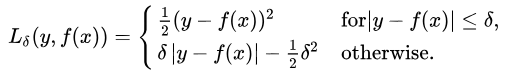
One thing we have to define here is the delta value. Delta is the hyperparameter that decides the range of MSE and MAE. When the error is less than the delta, the error is quadratic, otherwise absolute.
Delta can be iterative to find a correct delta value.
This equation says that, for a loss value less than delta, use the MSE. Use MSE when no outliers are present in the dataset. For loss value greater than delta, use the MAE.

Classification

Calculating the loss in classification is a little tricky.

Infobyte


What is entropy?


Entropy is a measure of the randomness, unpredictability, disorder, or impurity in a system.

Classification tasks are those in which the given data is classified into two or more categories.

For example, the classification of dogs and cats.

Types of Classification

In general, there are three main types/categories for Classification in machine learning:

A. Binary classification

This includes two target classes.
• Is it a cat in the picture? Yes or No

Object Target Prediction(Probability)
Yes 1 0.8
No 0 0.2

• Is it a cat or a dog in the picture? Cat or Dog

B. Multi-Class Classification
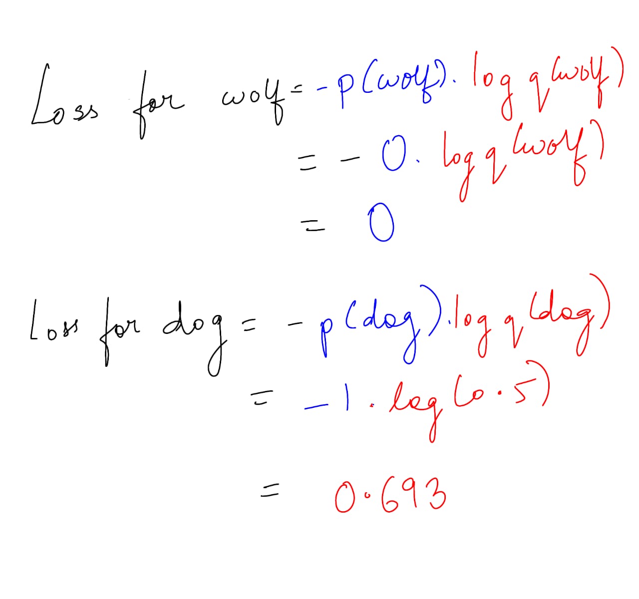
Classification

Object Target Prediction(Probability)
Dog 1 0.5
Cat 0 0.2
Wolf 0 0.3

The prediction of a model is a probability, and all these probabilities add up to 1. The target for multi-class classification is one hot vector, which means it has 1 on a single position and 0 everywhere else.

First, let us start calculating separately for each class and then sum it up.

loss function in classification

Loss function in Classification Loss function in Classification cross entropy

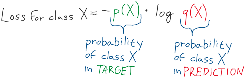
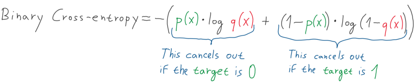
Binary entropy is a particular case of entropy used if our target is either 1 or 0. In a neural network, we achieve this prediction by using the Sigma activation function –

How to create a classifier – Check here.

Say I want to predict whether the image contains a cat or not.

Binary loss function

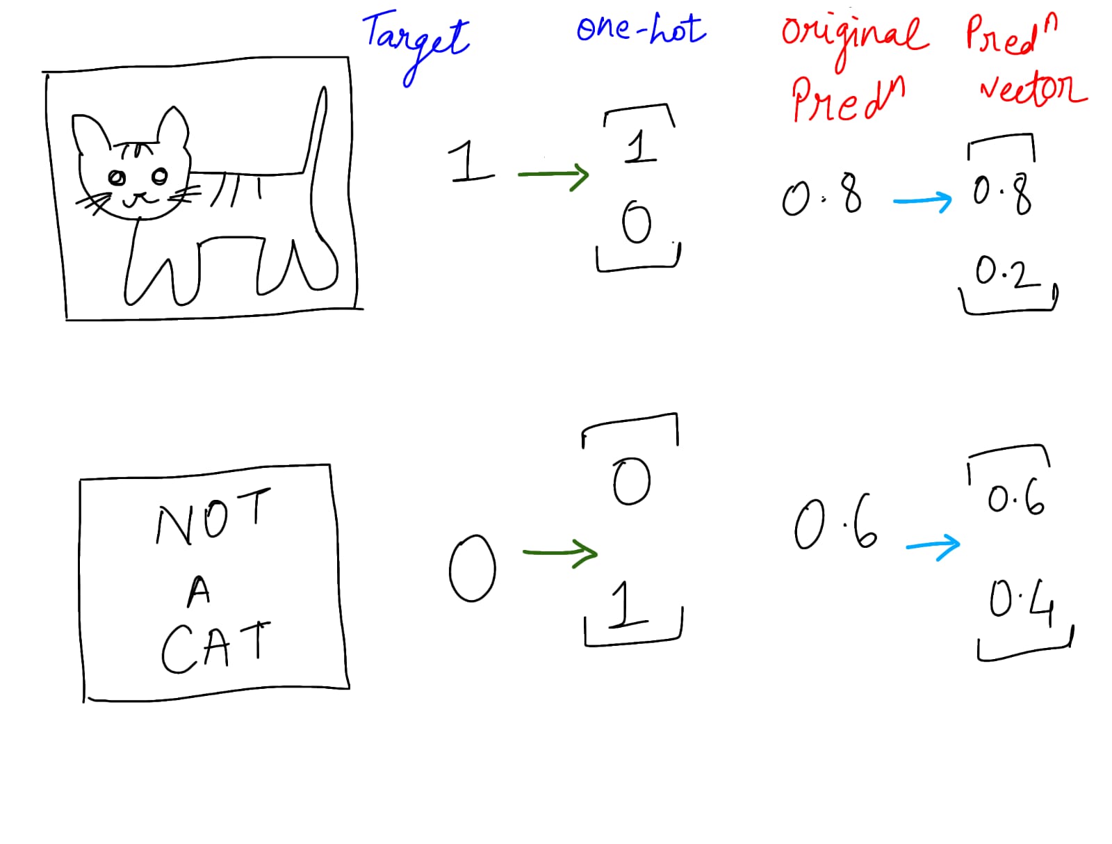
This is as simple as saying for 0.8 probability, which means 80 % it’s a cat and 20 % it is not a cat.

Binary cross entropy

C. Multi-label classification


In multi-label classification, an image can contain more than one label. Therefore, our target and predictions are not probability vectors. It’s possible that all the classes are present in one image, and even none at all sometimes.

Multi-label classification

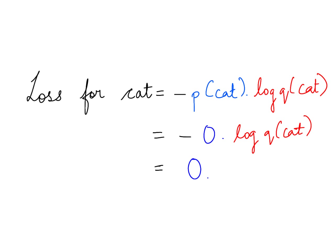
Here, we look at this problem as a multiple-binary classification subtask. Let us first predict if there is a cat or not.

loss function for classification


Done! Great work, you managed to read till here. Want some more exciting examples  – check here.

Authors:

Author of loss function in AI


Blog

Activation Function

Before we start with the activation function, let us quickly learn about a model. The article is a little longer because it has examples to make it simple for you to understand.


What is a model?

A model consists of 3 parts – input, actions on the input, and desired output.

We have input; we perform actions on it to get the desired output.

A model consists of input, action on input and output.

To know the basics of AI – click here


What is the activation function?

Girl crying due to burn 

An activation function is an action we perform on the input to get output. Let us understand it more clearly.

We all know that deep learning (DL), a part of Artificial Intelligence (AI) is a replica of the neural network in a human brain. For example, if you burn a little, you may/may not scream; if you burn terribly, you shout so loudly that the entire building knows.


Similarly, an activation function decides whether a neuron must be activated or not. It is a function used in DL which outputs a small value for small inputs and a large value if the input exceeds the threshold.

If the inputs are large enough (like a severe burn), the activation function activates, otherwise does nothing. In other words, an activation function is like a gate that checks that an incoming value is greater than a critical number (threshold).


Like the neuron-based model in our brain, the activation function decides what must be forwarded to the next neuron. The activation function takes the output from the previous cell (neuron) and converts it to input for the next cell.


Human Analogy

An old man giving chocolate

You see a senior citizen distributing free chocolates, your brain senses it as a tempting offer, and then it passes to the next neurons (legs) that you have to start running towards him(output from the preceding neuron).

Once you reach there, you will extend your hand to get the chocolate. So your output of every neuron is input for your upcoming action.


Why is activation function important?

The activation function in a neural network decides whether or not a neuron will be activated and transferred to the next layer. It determines whether the neuron’s input to the network is relevant or not for prediction, detection, and more.


It also adds non-linearity to neural networks and helps to learn powerful operations.


If we remove the activation function from a feedforward neural network, the network would be re-factored to a simple linear operation or matrix transformation on its input; it would no longer be capable of performing complex tasks such as image recognition.


Now let us discuss some commonly used activation functions.


1. Sigmoid Activation FunctionSigmoid Activation Function


Mainly used to solve non-linear problems. A non-linear problem is where the output is not proportional to the change in the input. We can use the sigmoid activation function to solve binary classification problems.

Consider an example,

Students appear for an examination, and the faculty designs an AI model to declare the results. They set criteria that students scoring more than 50 % percent are pass and below 50 % fail. So the inputs are the percentages, and the binary classification takes place using the sigmoid activation function.


If the percentage is 50 percent or above, it will give the output 1(pass)

Otherwise, it will give the output 0 (fail).


Output value – 0 to 1

If value >= 0.5, Output = 1

If value < 0.5, Output = 0

Derivative of sigmoid – 0 to 0.25.


What happens in the neural network?


A weight is assigned to input in the neural network. Different inputs have different weights. The weight is multiplied with the input, and at the next layer, all the products(w*x) are added.

Neural Network


∑wi*xi = x1*w1 + x2*w2 +…xn*wn


Based on these weights and activation, we get an output. Naturally, the system might make some mistakes while learning. (It might consider 55% as fail). In this case, to teach the system better, we take the derivative of the function and send it back to change the weights for correction. (Like a feedback mechanism)


Glance the formula for your understanding. Skip if it confuses you.

Neural Network new weight formula The derivative of the function is crucial for feedback mechanisms and corrections. Its range is only 0-0.25, which is a limitation for corrections. The feedback mechanisms and corrections are backward propagations. The outputs are considered as inputs to improve the accuracy.


Pros

  • Gives you a smooth gradient while converging, preventing jumps in output values.
  • One of the best Normalised functions.
  • Gives a clear prediction (classification) with 1 & 0; like pass/fail in above example.


Cons

  • Prone to Vanishing Gradient problem. The range of derivative is between 0-0.25, if used in deep neural networks, after some layers you will get very small values, and weights will not update. This problem is called the Vanishing Gradient problem. If your neural network has more hidden layers (it is deep) then this problem occurs easily.
  • Not a zero-centric function (Does not pass through 0).
  • Computationally expensive function (exponential in nature).


2. Tanh Activation Function

Tanh Activation function

Tanh is called a hyperbolic tangent function. Generally, used as the input of a binary probabilistic function. To solve the binary classification problems, we use the tanh function. In the tanh activation function, the range of the values is between -1 to 1. And derivatives of tanh are between 0 – 1.


Note – To solve the binary classification problem, we can use tanh for the hidden layer (to improve the vanishing gradient problem) and sigmoid for the output layer. However, the chances of a vanishing gradient remain.


Pros

• It is a smooth gradient converging function.

• Zero-centric function, unlike Sigmoid.


Cons

• Derivatives of tanh function range between 0-1. It is better than the sigmoid activation function but does not solve the vanishing gradient problem in backpropagation for deep neural networks.

• Computationally expensive function (exponential in nature).


3. relu Activation Function


Relu Activation Function  

Relu is Rectified linear unit; currently a more popular activation function. It solves linear problems. Range of values of ReLU: 0 – max.

ReLU = max(0 , x)

Derivatives of relu: 0 – 1.


Pros

• Deals with vanishing gradient problems.

• Computationally inexpensive function (linear in nature).

• Calculation speed much faster.


Cons

• If one of the weights in derivatives becomes 0, then that neuron will be completely dead during backpropagation.

• Not a zero-centric function.


4. Leaky ReLU Activation Function

Leaky Relu Activation Function

Use leaky relu to solve the dead ReLU problem. In leaky relu, the negative values will not be zero. The derivative will have a small value when a negative number is entered.

Leaky ReLU = max(0.01x , x)

As for the ReLU activation function, the gradient is 0 for all the values of inputs less than zero, which would deactivate the neurons in that region and may cause a dying ReLU problem.


Leaky ReLU is defined to address this problem. Instead of defining the ReLU activation function as 0 for negative values of inputs(x), we define it as an extremely small linear component of x. Here is the formula for the Leaky ReLU activation function


f(x)=max(0.01*x , x)


This function returns x if it receives any positive input, but for any negative value of x, it returns a small value that is 0.01 times x. Thus it gives an output for negative values as well. The gradient on the left side of the graph is a non-zero value. We no longer encounter dead neurons in that region.


Pros

  • To solve the dead neuron problem.


5. Elu Activation Function


Elu Activation Function

Elu is exponential linear units.

If x>0, then

Whenever the x value is greater than 0, we use the x value, else we apply the below function.

y = x ;  if x>0

y = α.(ex–1) ; if x<=0

Pros

• Gives smoother convergence for any negative value.


Cons

• Slightly computationally expensive because using of exponential value.


6. PReLU Activation Function

Prelu Activation Function

Parametric relu. PReLU has a learning parameter function that fine-tunes the activation function based on its learning rate (unlike zero in the case of RELU and 0.01 in the case of Leaky RELU).

If ax = 0, y will be ReLU’

If ax > 0, y will be Leaky ReLU

If ax is a learnable parameter, y will be PReLU


Pros

  • It has the learning parameter function which fine-tunes the activation function based on its learning rate (unlike zero in the case of RELU and 0.01 in the case of Leaky RELU).


7. Swish Activation Function


Swish Activation Function

Swish is a smooth continuous function, unlike ReLU, which is a piecewise linear function. Swish allows a small number of negative weights to propagate, while ReLU thresholds all negative weights to zero. It is crucial for deep neural networks. The trainable parameter tunes the activation function better and optimizes the neural network. It is a self-gating function since it modulates the input by using it as a gate to multiply with the sigmoid itself, a concept first introduced in Long Short-Term Memory (LSTMs).


Pros

• Deals with vanishing gradient problem.

• The output is a workaround between ReLU and sigmoid function which helps to normalize the output.


Cons

• Cannot find out derivatives of zero.

• Computationally expensive function (as of sigmoid).


8. Softmax Activation Function

Softmax is used for solving multiclass classification problems. It finds out different probabilities for different classes.

It is used in the output layer, for neural networks that classify the input into multiple categories.


Softmax Activation Function


Tips for beginners

Q – Which activation function solves the binary classification problem?

A – For the hidden layer, use ReLU/ PreLU/Leaky ReLu, and for the output layer, use the sigmoid activation function.


Q – Which activation function solves the multiclass classification problem?

A – For the hidden layer, use ReLU/PreLU/Leaky ReLu, and for the output layer, use the softmax activation function.


Well Done! You ended up learning till here.

For more activation functions – Click here

Authors

authors - Ankita Gotarne & Janvi Bhanushali

Blog

Image Classification

What is Image Classification?

Image classification means assigning labels to an image based on a predefined set of classes.

Practically this means that our task is to analyze an input image and return a label that categorizes the image. That label is always from a predefined set of possible categories.

For example – Check here.

Let us understand image classification through an analogy.

Explanation of image classification through the body parts example

In a fourth-standard classroom, teacher Smita is teaching organs of the body to students. The teacher will show the children an image of each organ and give a title/label for it. She will show an image of a heart and point out to students that this is the heart. Similarly, she will show images of all the organs with their labels. The teacher will repeat this exercise and do revisions until it is clear to the students which organ looks like what.

In image classification, we teach the system by showing images and labels of predefined categories.

How do we create image classification models? How do we teach the systems to classify the images accurately? 

We need to follow some steps to create an Image Classifier. Technically, we need to follow a classification pipeline to train the system to classify images.

Classification Pipeline

Image classification block diagram

The basic idea is to build an image classification model with Convolutional Neural Networks. We use a data-driven approach despite coding a rule-based algorithm to classify images. In a data-driven approach, we supply examples of what each category looks like and then teach our algorithm to recognize the difference between the categories using these examples.

We call these examples – the training dataset. It consists of images and labels associated with each image like {tom, jerry, spike}. 

It is crucial to give these examples to the system for supervised learning. These labels teach the system how to recognize each category. (Recall the organs of the body example – how the teacher points out which organ looks like what)

Now that we know what an image classifier model is. Let us understand how to create a Deep-Learning Image classifier model step-by-step.

Classification Pipeline:

Image Classification steps: 1. Collect Dataset 2. Split Dataset 3. Autotune 4. Train and Test

The classification pipeline has 5 steps: 

  1. Collect Data: collect and preprocess the raw data.  
  2. Split Data: split the preprocessed data into train, validation, and test data. 
  3. Autotune: find the best parameters on the validation data. 
  4. Train: train the final model with the best parameters on all the data. 
  5. Test: get metrics and predictions on test data. 

Step 1: Gather your Dataset

We need images and labels associated with each image. These images and their labels form our dataset. The labels should be from a finite and predefined set of categories like:

Categories – tom, jerry, spike.

Things to keep in mind:

  • The number of images from each category should be approximately uniform. Like 1000 images for Tom, 1000 for Jerry, and 1000 for Spike.
  • If we keep 2000 images for Jerry, our classifier will become naturally biased to this heavily represented category.
  • To prevent bias, avoid class imbalance and gather a uniform number of images for each category.

Step 2: Split Your Dataset

After gathering the initial data, we split it into two parts:

  1. A training set
  2. A testing set

A training set teaches our classifier what each category looks like. The classifier makes predictions on input data and then corrects itself if predictions are wrong.

After the classifier is trained, we evaluate the performance on a testing set.

You can split the training and testing set in the following ways:Pie Chart of train data and test data

Validation Set :

This data is from the training data and used as “fake test data” so we can tune our hyperparameters (Autotuning). We generally allocate 10%-20% of the training dataset for validation.

Step 3: Train Your Network

Once we are ready with all sets of the training data, we can start training our network. Our goal is to teach our neural network each category in our labeled data. When the model makes a mistake, it learns and improves itself.

Step 4: Evaluate

Last, we need to evaluate the performance of our trained network. We present each of the images in our testing dataset to the network and ask it to predict the label for that image. We tabulate the predictions of the trained model and compare them to the actual category of the image. Thus, we can determine the number of classifications our model got correct.

Image Classification Output

A deep-learning image classifier is ready, using a data-driven approach and supervised learning method. 

To create your own AI model – Click here

Authors:

Blog

Challenges in Image Classification

What is image classification?

Image classification means assigning labels to an image based on a predefined set of classes.

Practically, this means that our task is to analyze an input image and return a label that categorizes the image. The label is always from a predefined set of possible categories.
For example, let’s assume that our set of possible categories includes:
categories = {tom, jerry}

Our classification system could assign multiple labels to the image via probabilities, such as:

jerry: 95%; tom: 5% for the image on the left side.

jerry: 10%; tom: 90% for the image on the right side.

To learn how to create an image classifier – Click here

What are the challenges in image classification?

Below are the challenges that we face while doing image classification :

  1. Semantic gap: We can clearly see the difference between an image that contains a dog and an image that contains a cat. However, a computer sees a big matrix of numbers. The difference between how we perceive an image and how the computer sees the image(a matrix of numbers) is called the semantic gap.
Computer vision - how humans see and how computers see

Computer vision – difference between how humans see and computers see.

2. Viewpoint variation: Based on how the object is photographed and captured, it can be oriented in multiple dimensions.

Viewpoint Variation - a car captured from different angles

Viewpoint Variation – Same car from different angles

3. Scale variation: Have you ever ordered a small, medium,or large pack of fries at Mc Donald. They are all the same – a pack of fries, but of different sizes. Furthermore, the same pack of fries will look dramatically different when it is photographed up close versus when it is captured from farther away. The image classification methods must be tolerable to these types of scale variations.
Scale variation is a challenge of Image Classification

Scale Variation – Same pack of fries captured from different distances

4. Deformation : For those of you familiar with the television series Popeye, we can see Olive Oyl in the image. As we all know that Olive is elastic, stretchable, and capable of contorting her body in many different poses. We can look at these images of Olive as a type of object deformation – all images contain the Olive character; however, they are all dramatically different from each other.

Deformation is one of the challenges of Image Classification

  1. Occlusions: In the image on the left side, we have to have a picture of a cat. And in the image on the right side, we have a photo of the same cat. But how the cat is resting underneath the covers, occluded from our view. The cat is still clearly in both images – she’s just more visible in one image than the other. Image classification algorithms should still be able to detect and label the presence of the cat in both images.
    Image Classification Challenge - Occlusion

    Occlusion – The same object is more visible in one image

  2. Illumination: The image on the left side was photographed with standard overhead lighting while the image on the right side was captured with little lighting. We are still examining the same cupcake – but based on the lighting conditions, the cupcake looks dramatically different.

Background Clutter

Challenge of Image Classification - Illumination

Illumination – objects look different in different lighting

7. Background clutter: Ever played a game – to spot the bird? If so, then you know the goal of the game is to find the decided beautiful bird before the others. However, these games are more than just entertaining children’s game – they are also the perfect representation of background clutter. You can clearly see the Himalayan black-lored tit in the image on the left side. But the image on the right side is very noisy and has a lot of background clutter. We are interested in one particular object in the image; however, due to all the “noise”, it’s not easy to spot the bird. If it’s not easy for us to do, imagine how hard it is for a computer with no semantic understanding to spot it.

Image Classification challenge - Background clutter

Background clutter – The background noise makes it difficult to search the bird on the right side image

  1. Intra-class variation: The canonical example of intra-class variation in computer vision is displaying the diversification of dog breeds. We have different breeds of dogs some used for military, some as pets, some as guards – a dog is still a dog. Our image classification algorithms must be able to categorize these variations correctly.
    Intra-class variation is one of the challenges on Image Classification

    Intra-class variation – Different breeds of dogs

Watch this tutorial to create your own AI model – Click here

Authors:


Blog

History of Artificial Intelligence

Artificial Intelligence is not a concept of now, but of the ancient Greek times. The inanimate object can come to life is not just a concept in sci-fi movies, but is much older than you can imagine. There are myths of mechanical men and robots in ancient Greek and Egypt. However, John McCarthy coined the term Artificial Intelligence not before 1955. Let us glance through a brief history of AI:

History of AI - Alan Turing Test, AI program, John McCarthy, Eliza, Wabot, Boom of AI, World Chess Champion, 1st AI vacuum cleaner, AI in Netflix, Chatbot, Google Duplex.

What is AI? Check out this blog with exciting examples – Click here

Infobytes

Alan Turing TestTuring Test Description Artificial Intelligence

It is a test to determine whether a computer can think like a human being or not. 

It consists of three participants – a human evaluator(X) on one side and a human(A) and a computer(B) on the other side. If the evaluator (X) can’t recognize which candidate is human and which candidate is a computer after a series of questions, the computer successfully passes the Turing test. If the computer system successfully mimics the human, then it has passed the Alan Turing Test. 

To date, no AI has passed the Turing test, but some came pretty close.  

 
ELIZA – First Chatbot
Eliza - First Chatbot using Artificial Intelligence

The first chatbot

Bots are able to have human-like interaction because they are powered by two technologies – artificial intelligence and natural language processing that provides human-like intelligence to the bots.

ELIZA, aimed at tricking its users by making them believe that they were having a conversation with a real human being.

ELIZA operates by recognizing keywords or phrases from the input to reproduce a response using those keywords from pre – programmed responses.  For instance, if a human says that ‘My mother cooks good food’. ELIZA would pick up the word ‘mother’, and respond by asking an open- ended question ‘Tell me more about your family’. This created an illusion of understanding and having an interaction with a real human being though the process was a mechanized one.

 
WABOT
Robot - Wabot using Artificial Intelligence

First Robot – WABOT

This robot had hands and limbs that could extend and grab objects as well as legs that could walk in a rudimentary fashion. WABOT-1 also had semi-functional ears, eyes, and a mouth. The robot uses these sensory devices to communicate with a person in Japanese and estimate distances. Experts have estimated that WABOT had the mental faculty of a one-and-a-half-year-old child.

Computer beats the World Champion
World History - AI defeats human chess and becomes a champion

AI defeats the human opponent to become wold chess champion.

On May 11, 1997, an IBM computer called IBM Deep Blue beat the world chess champion after a six-game match: two wins for Deep Blue, one for the champion, and three draws. The match lasted several days and attracted massive media coverage around the world. It was the classic plot line of man vs. machine. It pushed forward the ability of computers to handle complex calculations needed to help discover new medical drugs; do broad financial modeling, identify trends, and do risk analysis; handle large database searches, and perform massive calculations needed in many fields of science.

This experiment formed the base for the upcoming parallel computing and Artificial Intelligent technologies.

 
Roomba – vacuum cleaner
First Vacuum Cleaner using Artificial Intelligence

First AI Vacuum Cleaner – Roomba

The battery-operated Roomba rolls on wheels and responds to its environment with the help of sensors and computer processing. When it bumps into an obstacle or detects an infrared beam, a boundary line the robot will change direction randomly.

 
Duplex
Google Duplex - AI assistant booking an appointment for haircut at a salon

Google Duplex

A technology that sounds natural to make customer experience comfortable. Duplex makes a phone call and arranges an appointment at a salon for the user. The receptionist at the salon doesn’t even realize that s/he was having a conversation with a machine(Duplex). 

The peak of AI is yet to come…

What are you waiting for? It is time to make your own AI model now – Click here

Author: